Explain the process of determination of equilibrium national income class 12
Looking for the process (method) of determination of equilibrium national income as per the syllabus of class 12 Macroeconomics CBSE Board.

Determination of equilibrium of national income is also known with various names as follows.
- Determination of short run equilibrium output.
- Determination of national employment.
As equilibrium of national income, output and employment coincide at the same point in the short run.

Let’s dive deep into this concept.
What is the meaning of Equilibrium level of Income
The equilibrium level is that likely level of income which has no tendency to change given the aggregate demand and aggregate supply in an economy.
As the study of the determination of equilibrium national income is only restricted to the short run. It is also the study of
- Determination of national output
- Determination of national employment.
Let’s discuss why all three studies are the same.
Why determination of equilibrium national income is also called determination of short run equilibrium output and employment.
See, to keep this economics concept simple for the class 12 students. The study of the equilibrium of national income is restricted to only a short run-time period.
What is Short run time Period.
Short run time period is the period, where technology does not play any role in the determination of the output in an economy. In other words, technology is constant.
Output is only determined exclusively by the level of employment in the economy.
It mean, output can be increased by increasing employment and vice-versa.
Note:- Here employment refers to the Human employment.
If employment is increased, output increases and the Income of the human employees also increases.
Hence, theses three economics variable, Income, output and employment shows same trend in short run and their equilibrium lie at the same point.
Thus, the study of determination of equilibrium of national income is also the study of determination of equilibrium of national output and employment.
Economic theory to study the Equilbrium National Income
The equilibrium of national income, output and employment can be studied by two theories.
- Classical Theory
- Keynesian Theory
But, we will study the Equilbrium of all three economic variable, i.e, income, employment and output as per the theory of Keynesian only.
Note:- Classical theory is not in the syllabus of Class 12 CBSE Board.
As per the Keynnesian Economics Theory
“As technology is assumed to be constant, there is one to one relationship between output and employment, . In the short run, output can only be increased by increasing employment and vice-varsa. Accordingly, output (GDP) can not be increased once there is full employment in the economy.”
Note:- There is no need to mention the name of theory while you answer this question. As there is no mention of Keynnesian theory in syllabus.
Determination of Equilibrium of Income (output)
In order to make the study of Equilibrium of income (output) simple for the class 12 students. Certain assumptions have been made.
Assumptions
It is a short run analysis:-
In order to keep study simple. The equilibrium of national income is studies in short run. It is assumed the technology is constant and output can only be increased by increasing employment and vice-versa.
The overall Price level in the economic is fixed:-
The overall level is the average price level of all the goods and services produced in the economy. By making this assumption the effects of change in price level on aggregate demand and aggregate supply are avoided.
The economy is a closed economy without government:-
It is assumed that the economy is the closed one. It does not have any relationship with rest of the world. Hence, there is no foreign trade, i.e., import and export.
It implies that there is no taxes and government expenditure in the economy. This eliminates government expenditure component of the aggregate demand.
Two Sector Model:-
The determination of equilibrium output is to be studies in the context of two sector model (households and firms). It implies no government and foreign trade.
Hence Aggregate Demand equals to
AD = C + I
Autonomous Investment:-
In order to keep study simple. It is assumed that level of investment is not influenced by the level of income. Investment is autonomous.
Two Approaches for Determination of Equilibrium level
The two approaches are
- Aggregate Demand – Aggregate Supply Approach (AD – AS Approach)
- Saving – Investment Approach (S – I Approach
How both AD-AS and S-I approaches are same
Both approaches are same. Saving and Investment approach can be derived from AD and AS approach. Both leads to the same conclusion.
Let’s have a look how they both are equal.
The equilibrium level of national income is determined at the point where aggregate demand (AD) equals aggregates supply (AS).
AD = AS —————- (i)
As, we have assumed that there is neither foreign trade nor government. Aggregate Demand AD is now reduced to the sum of private consumption expenditure (C) and Investment (I). Therefore,
AD = C + I ……………………(ii)
Aggregate supply is equal to the national income (Y). It is used either for consumption (C) or saving (S). It can be expressed as:
AS = C + S…………………..(iii)
Let’s show how both approaches are same.
putting (i), (ii) and (iii) together, we get:-
AD = AS
C + I = C + S
I = S or S = I
The above derivation shows, the basic approach AD = AS can also be expressed as S = I. It gives two approaches
- AD = AS
- S = I
Let’s discuss both approaches one by one.
Determination of Income by AD – AS approach
According to Keynesian theory, the equilibrium level of income in an economy is determined where Aggregate Demand AD is equal to the Aggregate Supply (AS).
AD = AS
Aggregate Demand (AD) comprises two components, Consumption, and Investment.
AD = C + I
to make study simple. Investment is assumed as autonomous (constant). Does not change with the change of level of income.
Aggregate supply is the total planned output and equal to national income. It comprises of two components.
AS = C + S
The curve of the AS is represented by a 45-degree line.
The determination of equilibrium level of income can be better understood with the help of the following schedule and diagram:-
| Employment (Lakhs) | Income | Consumption (C) MPC = 0.8 | Saving (s) MPS = 0.2 | Investment (I) | Aggregate Demand (AD) | Aggregate Supply (AS) | Effect on Income |
| 0 10 20 30 | 0 100 200 300 | 40 120 200 280 | – 40 – 20 0 20 | 40 40 40 40 | 80 160 240 320 | 0 100 200 300 | AD>AS AD>AS AD>AS AD>AS |
| 40 | 400 | 360 | 40 | 40 | 400 | 400 | Equilibrium AD = AS |
| 50 60 | 500 600 | 440 520 | 60 80 | 40 40 | 480 560 | 500 600 | AD<AS AD<AS |
Diagram of AD = AS Approach
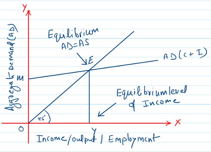
In the above diagram, AD shows the planned expenditure on consumption and investment as a given level of income.
The economy is equilibrium at point E where the AD curve intersects a 45-degree line (AS).
- E is the equilibrium level as per the above diagram. At this point planned expenditure equals to the level of output.
- OY is the equilibrium level of Income and output correspinding to point E.
- As the above table, Equilibrium of Income is at ₹ 400. At this income level AD is equal to AS.
- E, is the point of Effective Demand. Effective demand signifies the point where aggregate demand equals to aggregate supply. Thus, that level where aggregate demand equals aggregate supply is called Effective Demand.
What happens when AD > AS
Suppose AD is greater than AS. It means that buyers are planning to buy more goods and services than producers are planning to produce.
Producers keep a certain stock of goods called inventory. When AD is greater than AS, it means that buyers are buying faster than sellers are expecting.
In this situation, inventories start falling and come below the desired level. To bring back the inventories at the desired level producers expand production.
This raises the income level which keeps on rising till the AD and the AS once again become equal.
This brings the economy back to equilibrium.
What happens when AD < AS
Now, suppose that AD is less than AS. It means that buyers are planning to buy less than what sellers are planning to produce.
As a result, inventories start rising and move above the desired level.
As a result, the producers cut back on production and lay off workers.
This reduces the income level, i.e. AS. The downward trend continues till AD and AS once again become equal.
This brings the economy back to equilibrium.
Determination of Income by S = I Approach
According to this approach, the equilibrium level of income is determined at a level, when planned saving (S) ie equal to planned investment (I).
Let’s understand it with the following schedule and diagram.
| Income (Y) | Consumption (C) | Saving (S) | Investment (I) | Remarks |
| 0 100 200 300 | 40 120 200 280 | – 40 – 20 0 20 | 40 40 40 40 | S<I S<I S<I S<I |
| 400 | 360 | 40 | 40 | S = I |
| 500 600 | 440 520 | 60 80 | 40 40 | S>I S>I |
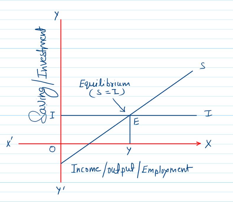
The investment curve is parallel to the X axis as it is not affected by the level of income. The saving curve slopes upwards show a positive relationship with income.
The economy is in equilibrium at point E, where planned autonomous investment is equal to planned savings.
OY is the equilibrium level of income and output corresponding to point E.
The equilibrium level of income as per the table is ₹ 400 crore. when ex-ante saving equals to ex-ante investment.
What happens when S < I
When planned saving is less than planned investment. It implies households are planning to buy more than what the producer is planning to produce.
As a result, planned inventory would fall below the desired level.
In order to bring the inventory back to the desired level, firms would plan to increase the production till saving and investment become equal to each other.
What happens When S > I
When planned saving is more than the planned investment. It implies households are planning to buy less than what the producer is planning to produce.
As a result, planned inventory would increase above the desired level.
In order to bring the inventory back to the desired level, firms would plan to reduce the production till saving and investment become equal to each other.
